Day2:梯度下降

梯度下降

主要目的是通过迭代找到目标函数的最小值，或者收敛到最小值。—-也可参考《An overview of gradient descent optimization algorithms》

基于day1的代价函数，梯度下降就是找到一个方法使得 J 快速由峰值到峰底，例如：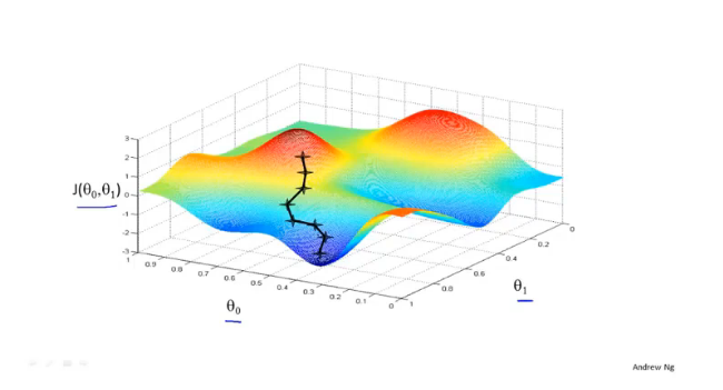

类似下山场景。 —《Gradient Descent - Problem of Hiking Down a Mountain》

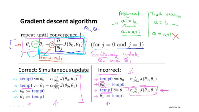
算法表示

代码实现

# 定义数据集和学习率
import numpy as np
# Size of the points dataset.
m = 20

# Points x-coordinate and dummy value (x0, x1).
X0 = np.ones((m, 1))
X1 = np.arange(1, m+1).reshape(m, 1)
X = np.hstack((X0, X1))

# Points y-coordinate
y = np.array([
    3, 4, 5, 5, 2, 4, 7, 8, 11, 8, 12,
    11, 13, 13, 16, 17, 18, 17, 19, 21
]).reshape(m, 1)

#--------------------------------------------------
#以矩阵向量的形式定义代价函数和代价函数的梯度
# The Learning Rate alpha.
alpha = 0.01

def error_function(theta, X, y):
    '''Error function J definition.'''
    diff = np.dot(X, theta) - y
    return (1./2*m) * np.dot(np.transpose(diff), diff)

def gradient_function(theta, X, y):
    '''Gradient of the function J definition.'''
    diff = np.dot(X, theta) - y
    return (1./m) * np.dot(np.transpose(X), diff)

#---------------------------------------------------
# 梯度下降迭代计算
def gradient_descent(X, y, alpha):
    '''Perform gradient descent.'''
    theta = np.array([1, 1]).reshape(2, 1)
    gradient = gradient_function(theta, X, y)
    #当梯度小于1e-5时，说明已经进入了比较平滑的状态，类似于山谷的状态
    #这时候再继续迭代效果也不大了，所以这个时候可以退出循环
    while not np.all(np.absolute(gradient) <= 1e-5):
        theta = theta - alpha * gradient
        gradient = gradient_function(theta, X, y)
    return theta

optimal = gradient_descent(X, y, alpha)
print('optimal:', optimal)
print('error function:', error_function(optimal, X, y)[0,0])

结果为：

optimal: [[0.51583286]
 [0.96992163]]
error function: 405.9849624932369

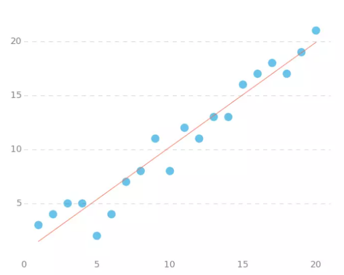
拟合结果为图中直线。

参考:

• 深入浅出—梯度下降法及其实现
• An overview of gradient descent optimization algorithms
• Gradient Descent - Problem of Hiking Down a Mountain